

Repulsive Curves – ACM Transactions in Charts
Curves play a fundamental role in computer graphics, physics simulation, and mathematical visualization, but most tools for curve design do nothing to avoid crossings or self-intersections. This paper develops efficient algorithms for (self-)repulsion of planar and spatial curves that adapt well to computational design problems. Our starting point is the so-called tangent point energy , which provides an infinite barrier to self-intersection. In contrast to the local collision detection strategies used, for example, In physical simulation, this energy considers the interactions between all pairs of points and is therefore useful for global shape optimization: local minima tend to be aesthetically pleasing, physically valid, and well-distributed in space. A reformulation of gradient descent, based on a Sobolev-Slobodeckij inner product, This allows us to progress rapidly towards local minima – regardless of curve resolution. We have also developed a hierarchical multigrade scheme that significantly reduces the cost per optimization step. Energy is easily integrated with a variety of constraints and penalties ( for example ,, (inextensibility or obstacle avoidance), which we use for applications including curve packing, node untangling, graph embedding, cross-spline interpolation, flow visualization, and robotic path planning.
PDF, 11MB
Video
|
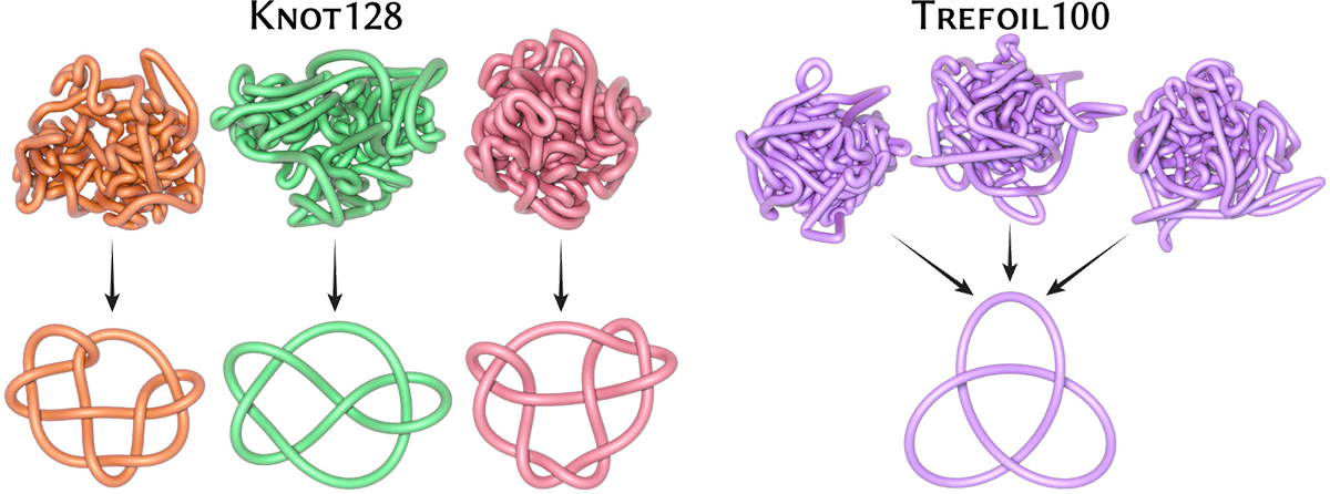
This file It contains two sets of data: Knot128 e Trefoil100 .Both datasets are “stress tests” for knot untangling algorithms, i.e., highly entangled configurations that can be difficult to smooth into a canonical knot embedding. Knot128 is composed of knots from 128 different isotope classes; for each class, we provide an entangled embedding and a canonical embedding (for reference). Trefoil100 contains 100 entangled embeddings of cloverleaf knot .To date, no algorithm – including ours – has been able to disentangle 100% from these nodes (see the article/supplement for statistics), although we come very close!
|
ZIP, 9.3 MB
|
repulsive-curves —Implementation C++, with interactive visualization via Polyscope .Curves and constraints can be specified by a simple "scene file," which is resolved to produce a sequence of optimized curves. Scenes support a wide variety of constraints and objectives, as described. here .
Additional
Supplementary Material — We conducted an extensive comparison with 19 alternative preconditioning and optimization methods, finding that, in general, the fractional Sobolev scheme performs significantly better than state-of-the-art optimization schemes for geometric energies. This paper also details how we generated our set of data from us .
|
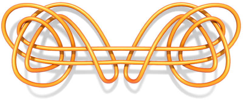
This file Contains meshes (at various resolutions) of the unknot from the article “Möbius Energy of Knots and Unknots” by Freedman, He and Wang, which is used as a performance benchmark in our article.
|
ZIP, 1.8 MB
|
Figures
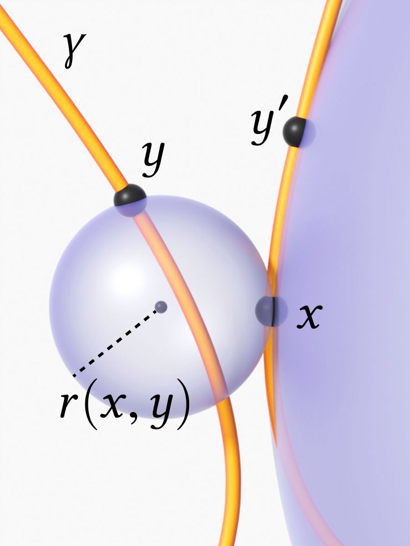
Our starting point is the tangential energy from Buck & Orloff (1995), that for each pair of points x e y In a curve, consider the radius. r of the smallest sphere tangent to x and passing through y .By penalizing the reciprocal of the ray 1/r(x,y) , Energy provides an infinite barrier to collisions – while naturally ignoring points that are close together in space simply because they are close along the curve itself.
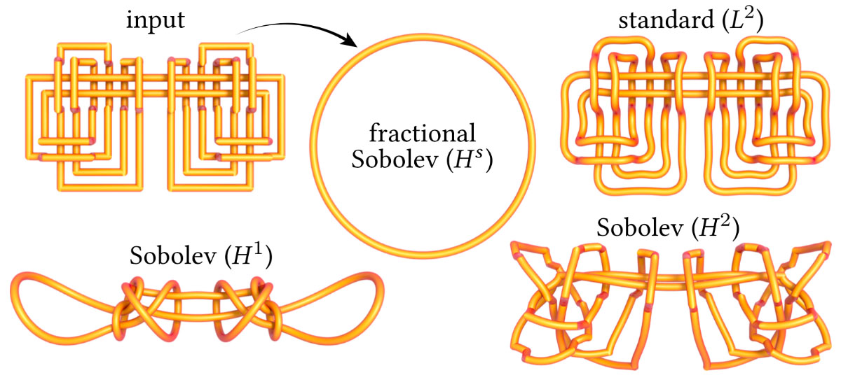
Untangling the highly tangled Freedman knot (top left corner) for the unit circle. For the same wall clock time, standard L2 gradient descent makes almost no progress, while conventional Sobolev descent fails to smooth low frequencies ( H 1 ) or high ( H 2 ). By carefully combining the inner product with energy, our fractional descent of Hs It flows quickly into the circle. .
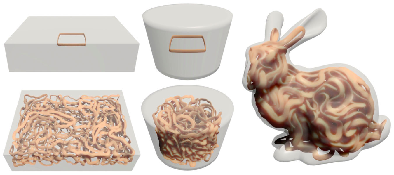
We can pack curves into a domain by penalizing their proximity to their boundary and progressively increasing the edge length. (Here we render curves with non-circular cross-sections, which are not modeled by energy.)
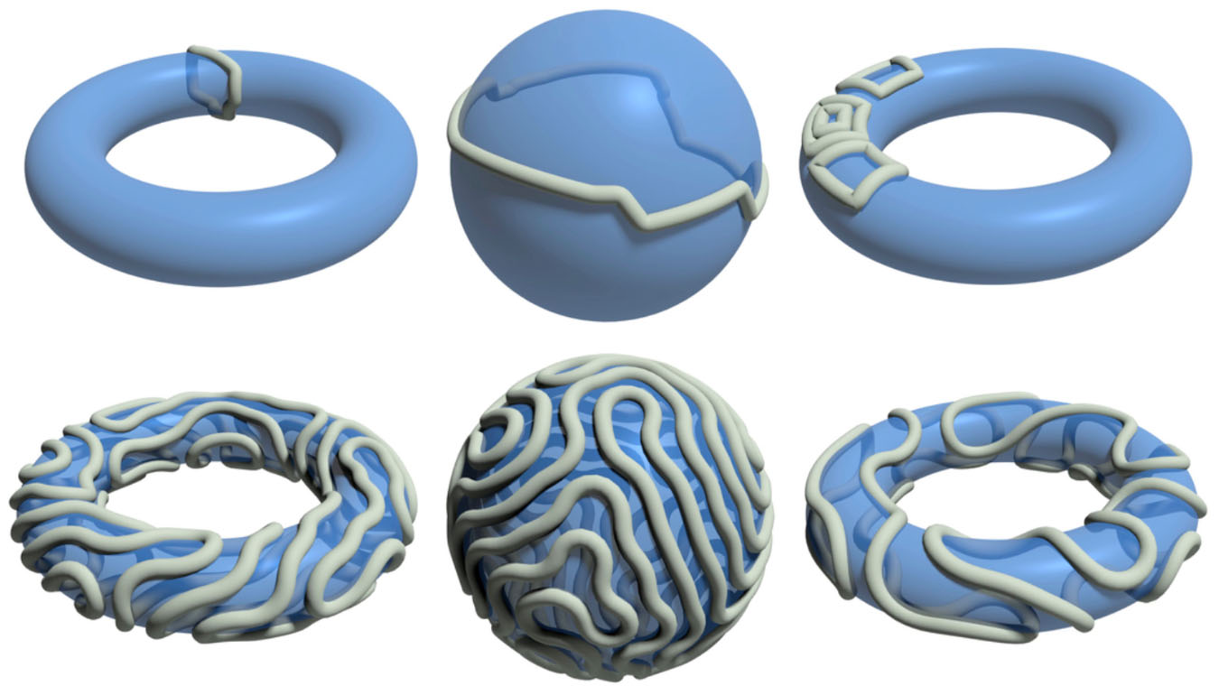
Patterns obtained by constraining a collection of repulsive curves to a surface and increasing their lengths (initial states shown above their final configurations).
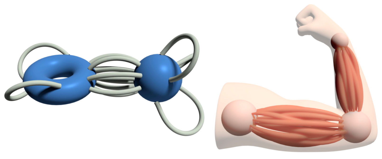
Allow the endpoints of the curve to slide freely over the constraint surfaces. (left) It allows for design tasks, such as organizing networks of muscles or muscle fibers. (right) .
Just as repulsive potentials are used to distribute points equally, we can calculate collections of equally spaced curves (here restricted to a region by means of a fixed curve potential).
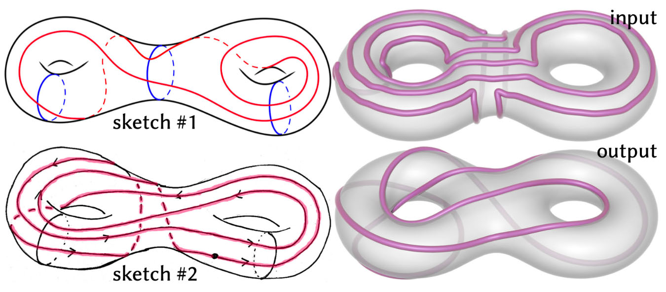
Topologically intricate loops can be difficult to draw by hand — the sketches on the left (drawn by Nathan Dunfield) illustrate the coordinates. Dehn-Thurston .On the right, we generate an equispaced version of this curve by flowing a rough sketch, subject to an implicit surface constraint.
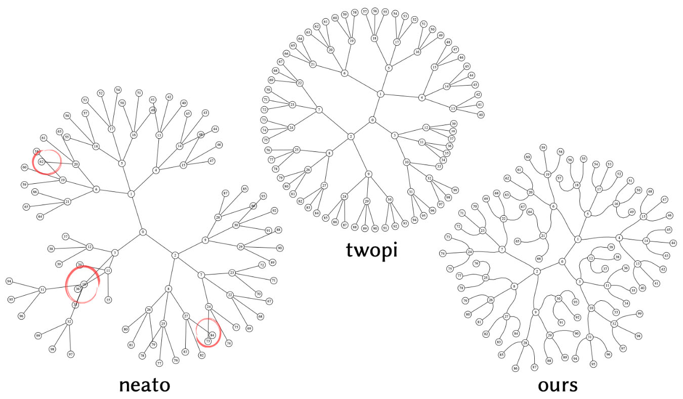
Traditional 2D graphing algorithms based on nodal proximity can cause edges to intersect. (left) or position the nodes extremely close together (center) ;These layouts were produced by the popular library. Graphviz. . By treating edges as repulsive curves, we can obtain graphic designs that are more compact and more legible. (on the right) .
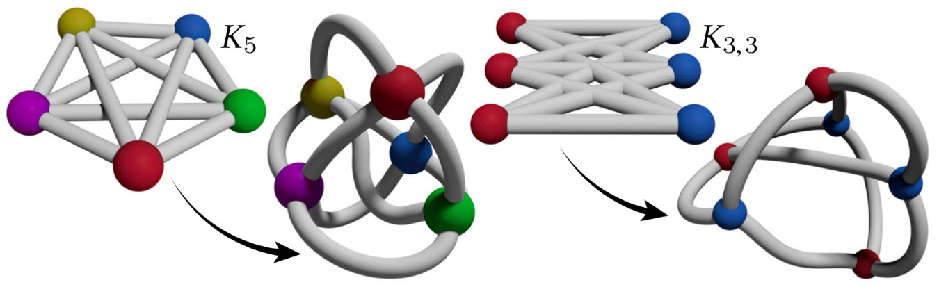
Isometric embedding: due to 2D jitter drawings of non-planar graphs (which necessarily have intersections), curve repulsion with length constraints produces well-spaced embeddings in R 3 with prescribed edge lengths.
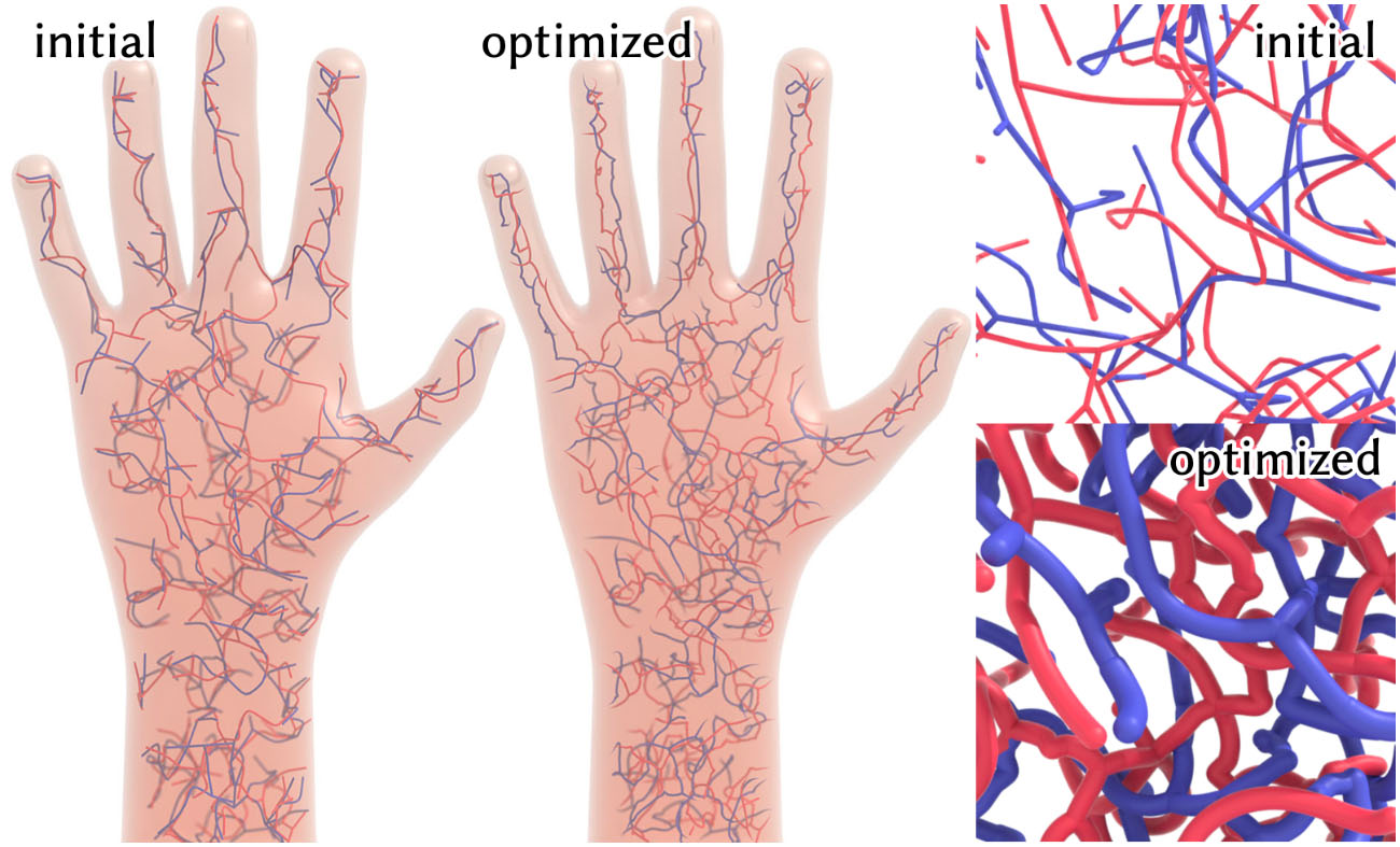
Left: A rough initial topology for a synthetic vascular network is optimized to achieve a more uniform distribution of nutrients in a volume. Right: Plotting the maximum thickness without collisions helps visualize the improvement in uniformity.
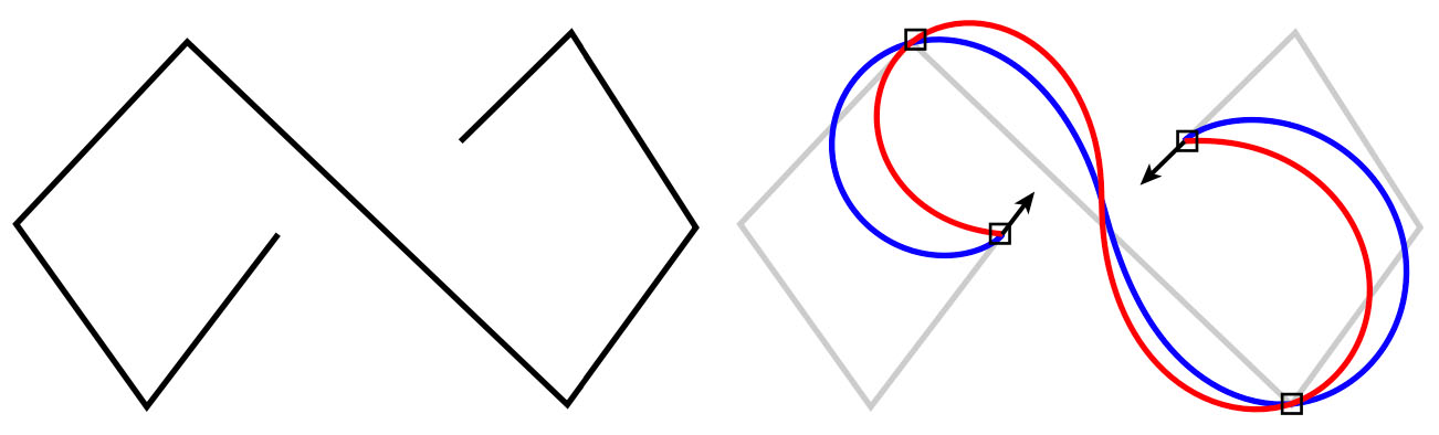
Just like with Bézier curves, we can also control the tangents of the curves both inside and at the ends. Here we are drawing a polygonal curve. (left) , for smooth interpolation with fixed points (red) and fixed points and tangents (blue) .
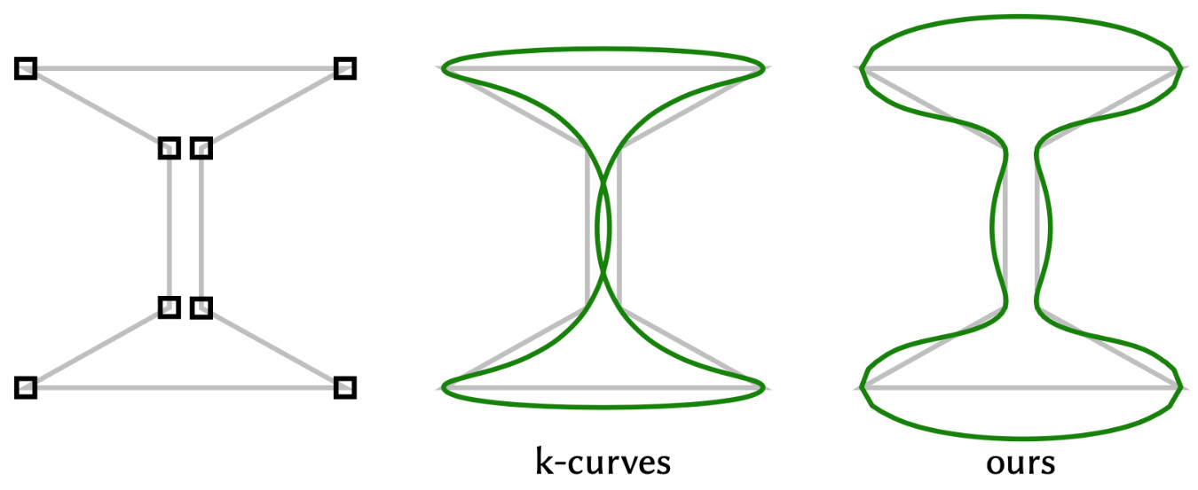
Standard curve interpolation methods in 2D drawing programs can cause curves to intersect automatically. (center) , even when the control polygon (left) No. Starting from the control polygon and restricting the control points, we obtain a smooth, intersectionless interpolator. (right) .
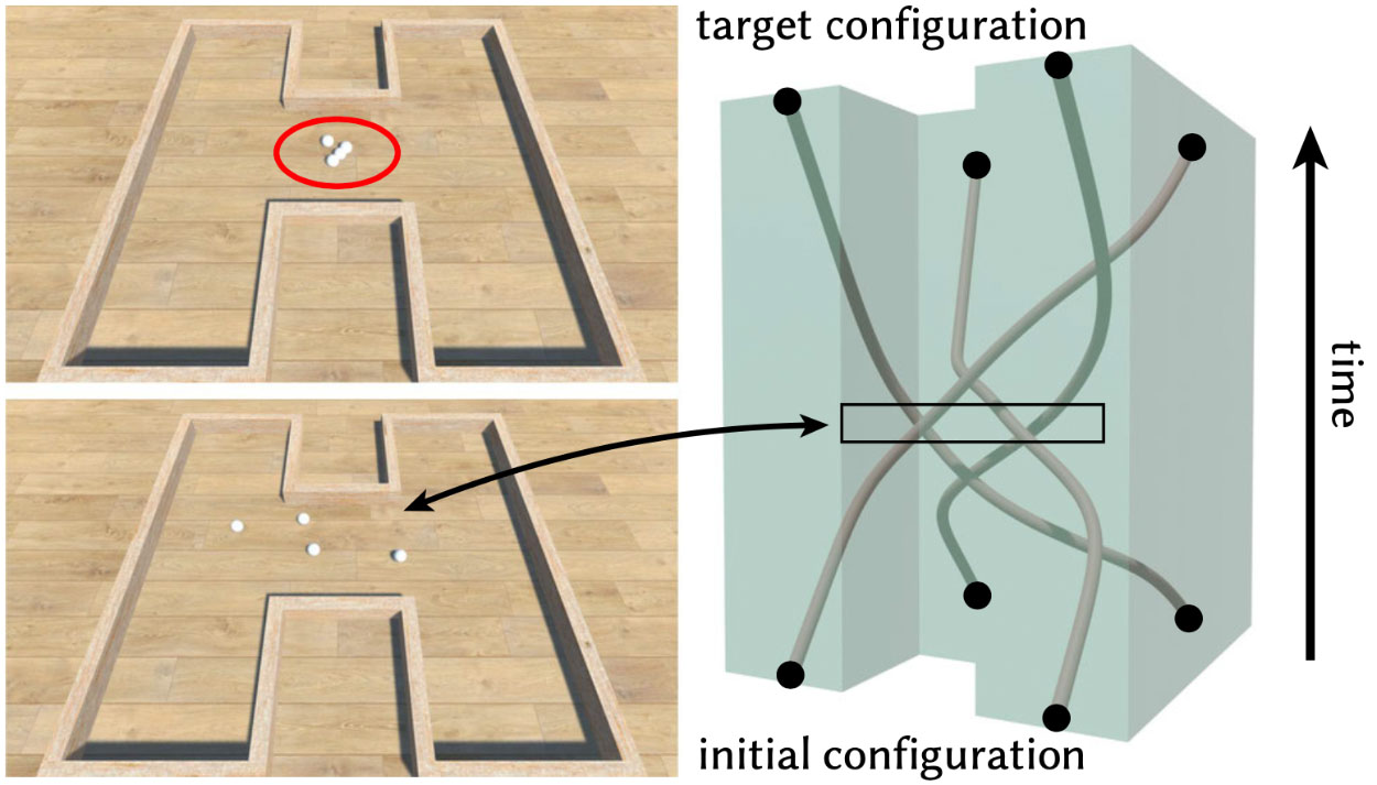
Top left corner: In this path planning scenario, an initial trajectory brings the four agents dangerously close together. Bottom left: By treating trajectories as curves in spacetime, our system provides solutions that avoid collisions as much as possible, making them more robust for error control. Right: Finding 2D trajectories is equivalent to optimizing a 3D braid with fixed ends constrained to an extrusion of a given environment. This same construction can be easily generalized to 3D environments.
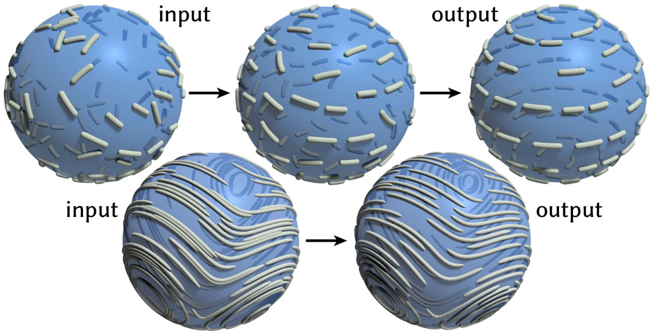
Encouraging curve tangents to align with a given vector field improves the quality of the simplified visualization. Here, a random set of curve segments is shown. (top) It aligns with a rotational vector field; we can also optimize randomly sampled flow lines. (bottom part) to improve your spacing.

Untangling a pair of headphones via repulsion (see supplementary video).
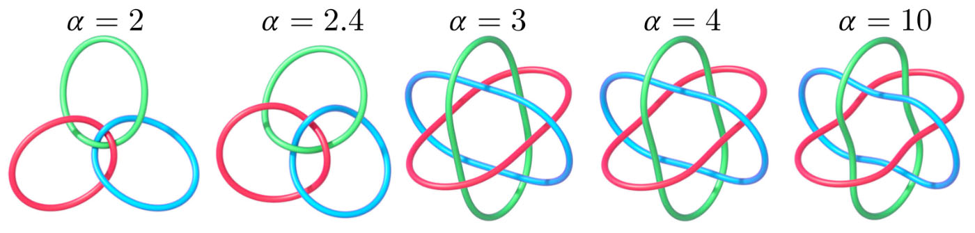
Local minimizers of the tangent point energy E 2α .When α = 2, the energy of the tangent point is scale-invariant and can exhibit "tight points"; for larger values of α, local interactions are more penalized than distant ones.
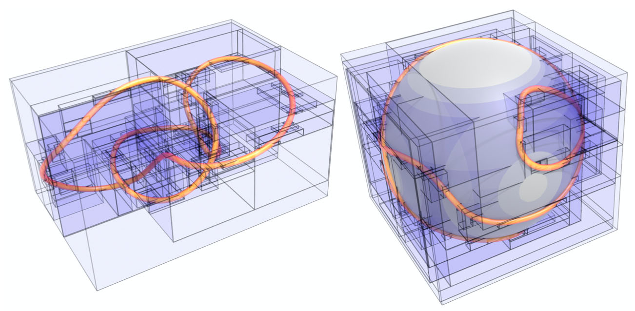
To speed up the evaluation of the tangent point energy, we constructed a bounding volume hierarchy that divides both positions. (left) and tangent directions (right) , depicted here as a curve on the unit sphere.


